A simple linear regression with TensorFlow 2.0
- 4 minsLinear regression
A very simple approach to perform a linear regression with a single neuron using Keras.
Package import
import tensorflow as tf
import numpy as np
import matplotlib.pyplot as plt
plt.style.use("ggplot")
Random data generation
We create our samples.
x = np.linspace(0, 50, 51)
x
array([ 0.,  1.,  2.,  3.,  4.,  5.,  6.,  7.,  8.,  9., 10., 11., 12.,
       13., 14., 15., 16., 17., 18., 19., 20., 21., 22., 23., 24., 25.,
       26., 27., 28., 29., 30., 31., 32., 33., 34., 35., 36., 37., 38.,
       39., 40., 41., 42., 43., 44., 45., 46., 47., 48., 49., 50.])
And for each sample add some random noise for the $y$ value.
y = x + 10 * np.random.random((len(x)))
y
array([ 4.59333333, 10.1888939 ,  3.10342612,  3.78295369, 10.57957367,
        8.31186454, 11.97466834,  8.38350117, 14.58165746, 12.7179244 ,
       16.04800824, 16.04253531, 17.7570093 , 15.36504093, 23.32077078,
       19.38063338, 25.72030949, 20.81364232, 18.55875267, 25.1340618 ,
       28.48036   , 21.73467374, 30.81790828, 28.56736033, 28.83225669,
       28.18684725, 34.95836113, 29.90731219, 30.90521404, 38.67280311,
       33.28501437, 40.01292045, 33.16216509, 34.99748693, 35.87077378,
       35.66317699, 36.37898628, 42.26194454, 47.36216501, 45.62434907,
       46.47169133, 48.05329522, 45.83970327, 50.68483177, 53.01284414,
       54.96997999, 46.42993498, 50.41667051, 53.26256812, 58.97071734,
       55.3635401 ])
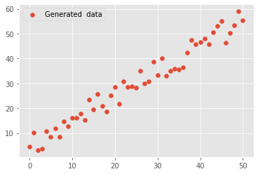
The generated data looks like this:
plt.figure(figsize=(10, 6), dpi=300)
plt.scatter(x, y, label="Generated  data")
plt.xlabel("Feature X")
plt.ylabel("Value y")
plt.legend()
plt.show()
Modelling
The model has just a single neuron that will model the linear equation $y = mx + b$.
The trained weight will correspond to the slope $m$ of the equation and the bias to the intersection value $b$.
model = tf.keras.Sequential()
model.add(tf.keras.layers.Input(shape=[1]))
model.add(tf.keras.layers.Dense(1))
model.compile(loss="mean_squared_error", optimizer=tf.keras.optimizers.Adam(0.1))
model.summary()
Model: "sequential"
_________________________________________________________________
Layer (type)                 Output Shape              Param #
=================================================================
dense (Dense)                (None, 1)                 2
=================================================================
Total params: 2
Trainable params: 2
Non-trainable params: 0
_________________________________________________________________
We proceed to fit the model.
history = model.fit(x, y, epochs=200)
Epoch 1/200
2/2 [==============================] - 0s 4ms/step - loss: 653.8051
Epoch 2/200
2/2 [==============================] - 0s 2ms/step - loss: 399.1392
Epoch 3/200
2/2 [==============================] - 0s 2ms/step - loss: 205.5257
Epoch 4/200
2/2 [==============================] - 0s 2ms/step - loss: 83.4503
Epoch 5/200
2/2 [==============================] - 0s 2ms/step - loss: 23.8983
[... 190 epochs omitted ...]
Epoch 196/200
2/2 [==============================] - 0s 2ms/step - loss: 8.8897
Epoch 197/200
2/2 [==============================] - 0s 2ms/step - loss: 8.8889
Epoch 198/200
2/2 [==============================] - 0s 1ms/step - loss: 8.8904
Epoch 199/200
2/2 [==============================] - 0s 2ms/step - loss: 8.8932
Epoch 200/200
2/2 [==============================] - 0s 2ms/step - loss: 8.9216
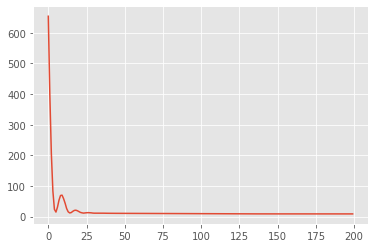
And we can plot the loss during the training.
plt.figure(figsize=(10, 6), dpi=300)
plt.plot(history.history["loss"], label="Training loss")
plt.xlabel("Epochs")
plt.ylabel("Loss")
plt.legend()
plt.show()
Model prediction
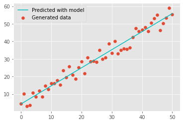
There are two ways to generate the adjusted model. The first one will be simlpy to use the .predict() method directly over the $x$ samples:
y_pred_model = model.predict(x)
plt.figure(figsize=(10, 6), dpi=300)
plt.scatter(x, y, label="Generated data")
plt.plot(x, y_pred_model, label="Predicted with model", color="c")
plt.xlabel("Feature X")
plt.ylabel("Value Y")
plt.legend()
plt.show()
The second (and my favorite) way is to understand the guts inside the network and access the information to literally replicate the model.
In this case we acces the first (and only) layer:
layer = model.get_layer(index=0)
layer
<tensorflow.python.keras.layers.core.Dense at 0x7fe81910e828>
Then, we get and print the weights and biases:
weights = layer.get_weights()
weights
[array([[1.0214125]], dtype=float32), array([4.3216815], dtype=float32)]
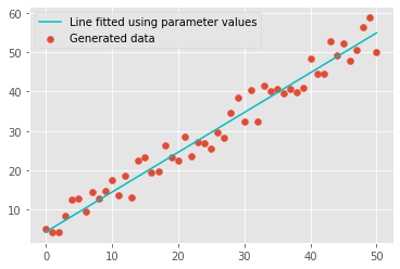
As we previously mentioned, the only weight will correspond to the slope and the bias to the intersection point. In order to replicate the linear equation we simply do:
m, b = weights[0][0], weights[1]
print(m)
print(b)
[1.014319]
[4.2396894]
y_pred_params = m * x + b
y_pred_params
array([ 4.23968935,  5.25400829,  6.26832724,  7.28264618,  8.29696512,
        9.31128407, 10.32560301, 11.33992195, 12.35424089, 13.36855984,
       14.38287878, 15.39719772, 16.41151667, 17.42583561, 18.44015455,
       19.4544735 , 20.46879244, 21.48311138, 22.49743032, 23.51174927,
       24.52606821, 25.54038715, 26.5547061 , 27.56902504, 28.58334398,
       29.59766293, 30.61198187, 31.62630081, 32.64061975, 33.6549387 ,
       34.66925764, 35.68357658, 36.69789553, 37.71221447, 38.72653341,
       39.74085236, 40.7551713 , 41.76949024, 42.78380919, 43.79812813,
       44.81244707, 45.82676601, 46.84108496, 47.8554039 , 48.86972284,
       49.88404179, 50.89836073, 51.91267967, 52.92699862, 53.94131756,
       54.9556365 ])
plt.scatter(x, y, label='Generated data')
plt.plot(x, y_pred_params, label='Line fitted using parameter values', color='c')
plt.legend()
plt.show()
If you want to run the code above directly on Google Colab, please follow this link.

Rodolfo Ferro
With great power comes great responsibility.